Fitting mixed models in Python with ASReml-R

NOTE: If you want to run the code examples in this tutorial you will need to have the following software installed.

• Python https://www.python.org/downloads/
• Jupyter notebook https://jupyter.org
• R https://www.r-project.org/
• A licensed version of ASReml-R (note: this is not free software) https://vsni.co.uk/software/asreml-r

Additionally you will need Internet access to open some of the Python packages and use the ASReml-R license.

Python is the most popular programming language for data science and related fields. It is versatile, user friendly, well documented and is backed by a vast and ever-increasing community. In addition, its libraries often have more permissive terms of licensing, and this generates significant interest, especially from industry.

If you are a Python user you might have noticed that despite the myriad of available libraries and frameworks - especially on the Machine Learning side - this language still lacks depth on some conventional, well-established and proven statistical tools, such as linear mixed models (LMMs).

LMMs have been around for decades, and they are the reference statistical method to analyse unbalanced, heterogeneous, correlated, and complex experimental data. This makes it a critical tool for applications in agriculture, ecology, food science, and genomics, to name a few fields.

In R we have some great libraries that can fit LMMs (and many other statistical models) that are missing in Python. Among the R libraries that can fit complex mixed models is ASReml-R (or simply, asreml). This package, and its stand-alone counterpart ASReml-SA, have been a popular choice for decades due to flexibility, efficiency, and reliability.

This tutorial will show you how to exploit the available tools in R. We will use the R library ASReml-R to demonstrate how to navigate between R and Python effortlessly.

To begin, we will present two ways to facilitate this interaction:

1. An R-focused approach, where we explicitly call ASReml-R with R code in between Python code sections; and
2. A Python-focused approach (a bit trickier), where we import and load ASReml-R as an internal Python library.

Note that these two are not the only ways to use R and Python together; we are merely demonstrating some possibilities and caveats so you can get started. Now, fire up a Jupyter notebook and follow along.

Installing rpy2

In both strategies we are going to use Python’s rpy2 library as the interface between Python and R. Run the following code to install rpy2 if you haven’t already.

!pip install --quiet pandas rpy2

Approach 1: calling ASReml-R with R code in between Python code sections

To get going with this approach first we need to load the packages: pandas and rpy2.

• pandas is a library to manipulate data frames, and
• rpy2 is an interface library to R embedded in a Python process.

import pandas as pd
import rpy2

We activate the R interface that will help us interact with the R code.

%load_ext rpy2.ipython

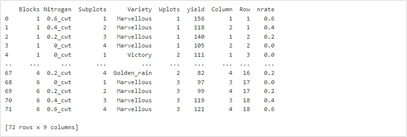
Now we are ready! In this example we will load the oats dataset into Python directly from a file then explore it further. Note that below we are only using Python code.

oats = pd.read_csv('https://downloads.vsni.digital/a984bcc71ddb47586c9cb67b49d7e3e5c4a820b3/oats.dat', sep = '\t')
print(oats)

To declare a notebook cell that uses R directly, we need to add the %%R command. Let’s try this by first loading the library ASReml-R that we will use for fitting our linear mixed models.

%%R
library(asreml)

Before we fit our models, we need to transfer the data (in this case oats) from Python to R, so we can make it available for the library ASReml-R.

To do this use the -i code after the %%R command, followed by the name of the data to be transferred. After executing this line we can perform any desired manipulations as we do with R, such as defining the class of variables. This is shown in the code below.

%%R -i oats
oats$Variety <- as.factor(oats$Variety)
oats$Nitrogen <- factor(oats$Nitrogen, levels = c('0_cwt', '0.2_cwt', '0.4_cwt', '0.6_cwt'))
oats$Blocks <- as.factor(oats$Blocks)
oats$Wplots <- as.factor(oats$Wplots)

Before we start our modelling within ASReml-R, we need to define our statistical model. For the oats dataset, we have a split-plot design with blocks with two main factors  (in whole-plots) and  (in sub-plots), and its linear model is:

where:

• is the response variable;
• , , and are the main fixed effect factors and their interaction;
• and are random blocking terms; and
•   is the random residual term.

The above model can be fitted with ASReml-R as follows:

%%R
oats_asr <- asreml(
fixed = yield ~ Variety + Nitrogen + Variety:Nitrogen,
random = ~Blocks + Blocks:Wplots,
residual = ~idv(units),
data = oats)

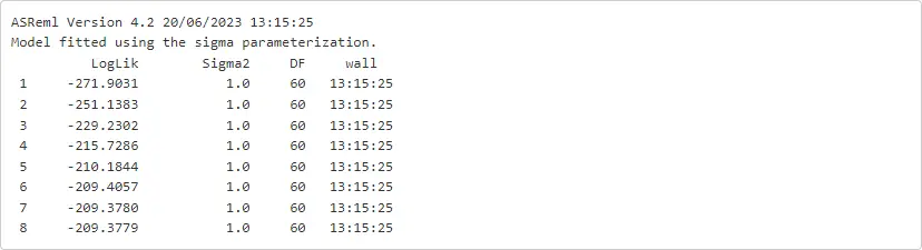
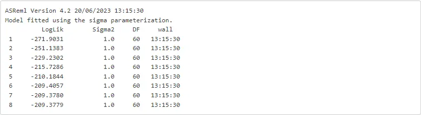
We might as well ask for additional iterations over the previous model using the function update.asreml. Note that the fitted model object was called oats_asr.

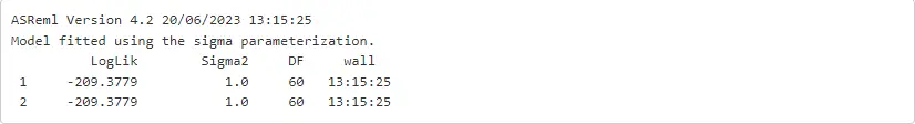
%%R
oats_asr <- update.asreml(oats_asr)

Before, we look into the estimates of the mode, we should check the model assumptions by exploring some diagnostic plots.

%%R
plot(oats_asr)

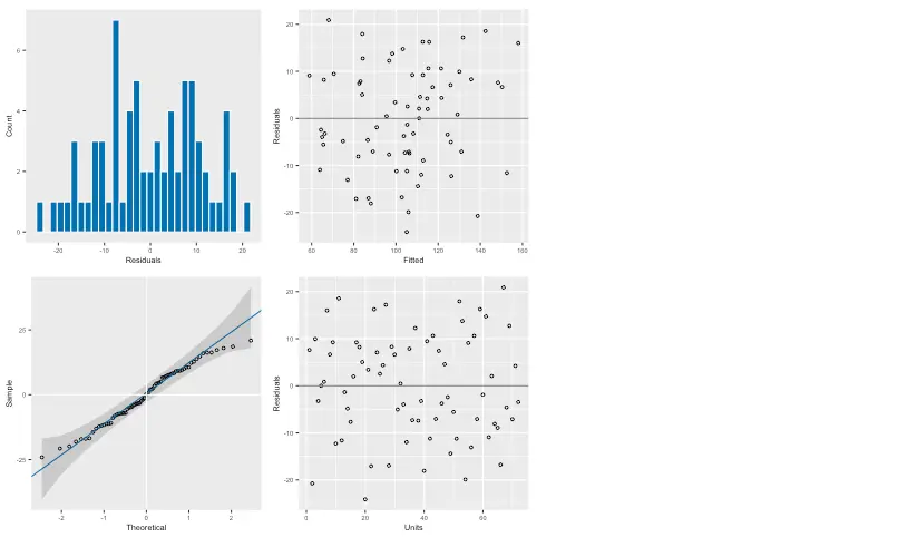
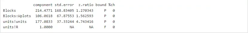
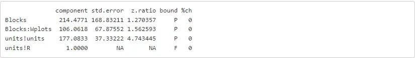
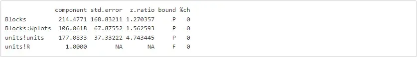
These seem reasonable, so now we can proceed to request the estimated variance components.

%%R
summary(oats_asr)$varcomp

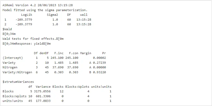
Also, we can invoke the wald.asreml function to get an ANOVA-like table to assess the significance of our main and interaction fixed effects. The comand below will provide the correct degrees of freedom associated with this experiment (i.e., split-plot), and the approximated F-tests are conditional with respect to all other terms in the model.

%%R
wald.asreml(oats_asr, denDF = 'numeric', ssType = 'conditional')

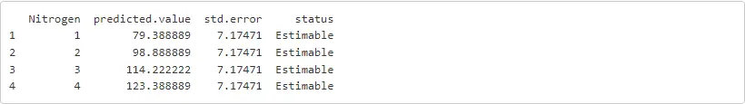
We can also use any other functions included in ASReml-R. Probably, one of the most interesting is the predict.asreml function that provides us with ‘estimated means’ of each fixed effect term of interest. In the code below, we are requesting these means for each level of Nitrogen.

Note that we are using the -o option to export the object preds from R into Python, and this will be defined as a pandas data frame.

%%R -o preds
preds <- predict(oats_asr, classify = 'Nitrogen')$pvals

And now preds is in Python! And it can be treated as other pandas object for further manipulations or explorations.

print(preds)

For this approach it was clear that Python and R are kept mostly separated in terms of environments and coding. However, the transfer from one to the other (both directions) is easily done with the rpy2 library. Hence, the capabilities of ASReml-R or any other R functions and/or libraries can be safely implemented along with our Python code.

Approach 2: import and load ASReml-R as an internal Python library

This approach might seem be a bit more familiar for Python users, but there are a few caveats to keep in mind, for example, the usage of dots (.) in functions and object names. This is very common in R, but in Python these are conflictive; hence, for compatibility, all dots need to be replaced by underscores (_). For illustration, instead of using summary.asreml we will have to use summary_asreml. Nevertheless, one important advantage is that we now can ignore all of the R code, and use just plain Python code.

To get going with this approach, first we need to import some required packages.

• rpy2 and pandas libraries (as we did in the previous approach),
• importr function used to import R packages,
• Formula function (as f for convenience) to write R formulas from strings, and
• pandas2ri function to enable automated conversion between pandas objects to R object. Note that this has to be activated.

The code required for the above elements is shown next.

import rpy2
import pandas as pd
from rpy2.robjects.packages import importr
from rpy2.robjects import Formula as f
from rpy2.robjects import pandas2ri
pandas2ri.activate()

We proceed to import the R library ASReml-R (named asreml) using the importr function.

asreml = importr('asreml')

Now, ASReml-R can be used as if it was any Python library, and its functions can be accessed via the code asreml.<function name> (just as for R using asreml::<function name>).

As an illustration, let’s import the oats dataset and do some testing.

oats = pd.read_csv('https://downloads.vsni.digital/a984bcc71ddb47586c9cb67b49d7e3e5c4a820b3/oats.dat', sep = '\t')

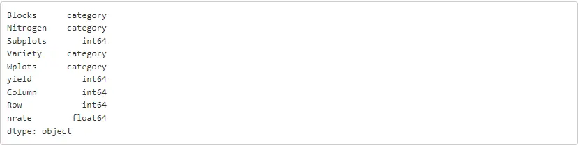
For Python, if some of the variables have to be transformed into categories ('factors' in R lingo), this can be done using the astype() and CategoricalDtype() functions. This is done below, and we also use oats.dtypes to check the type of each column.

oats['Variety'] = oats['Variety'].astype('category')

oats['Nitrogen'] = oats['Nitrogen'].astype(
pd.CategoricalDtype(categories = ['0_cwt', '0.2_cwt', '0.4_cwt', '0.6_cwt'], ordered = True))

oats['Blocks'] = 'B' + oats['Blocks'].astype(str)
oats['Blocks'] = oats['Blocks'].astype(
pd.CategoricalDtype(categories = ['B1', 'B2', 'B3', 'B4', 'B5', 'B6'], ordered = True))

oats['Wplots'] = 'W' + oats['Wplots'].astype(str)
oats['Wplots'] = oats['Wplots'].astype(
pd.CategoricalDtype(categories = ['W1', 'W2', 'W3'], ordered = True))

print(oats.dtypes)

The linear mixed model that was defined for approach 1, based on a split-plot design with blocks, can now be fitted with ASReml-R as shown below. Note that all results are sent to the object oats_asr.

oats_asr = asreml.asreml(
fixed = f('yield ~ Variety + Nitrogen + Variety:Nitrogen'),
random = f('~Blocks + Blocks:Wplots'),
residual = f('~idv(units)'),
data = oats)

There are a few comments related to this code cell.

• The asreml.asreml code calls the asreml function (second word) from the asreml package (first word).
• The Python function f is being used to transform the strings into R formulas. This is required as Python does not have an equivalent class.
• The oats data set is being automatically converted into an object of a class that ASReml-R can use.

We can now check the outputs by having a look at the oats_asr object. For example, below we print the estimated variance components.

summ = asreml.summary_asreml(oats_asr)[4]
print(summ)

rpy2, rx and rx2 are used as proxies for R operators [] and [[]] respectively. Hence, to get the variance components from the fit model we can run:

summ = asreml.summary_asreml(oats_asr)
print(summ.rx2('varcomp'))

We hope this short tutorial has provided you with sufficient information on using ASReml-R alongside Python. It is important to note that ASReml-R was  primarily designed, optimised, tested, and supported for R. Therefore, certain parts of the code may require additional techniques or workarounds when using it with Python. We would appreciate hearing about your experience using ASReml-R with this R/Python interface. Please feel free to share your feedback with us at support@vsni.co.uk.

Appendix

The session information is reproduced below for reference.

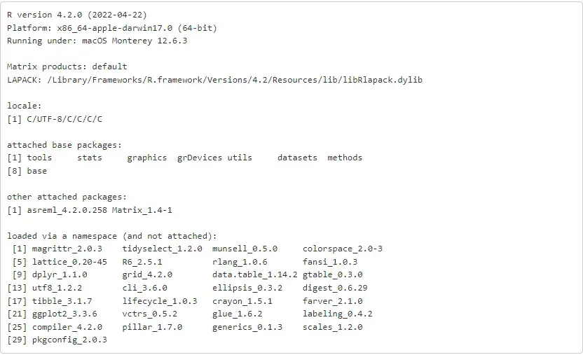
%%R
sessionInfo()

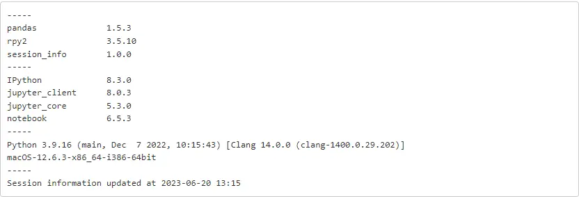
import session_info
session_info.show(excludes = ['asreml'], html = False)

About the author

Dr. Giovanni Galli is an Agronomist with an M.Sc. and Ph.D. in Genetics and Plant Breeding from the University of São Paulo (USP)/Luiz de Queiroz College of Agriculture (ESALQ). He currently works as a Statistical Consultant at VSN International, United Kingdom. Dr. Galli has experience in field trials, quantitative genetics, conventional and molecular breeding (genomic prediction and GWAS), machine learning, and high-throughput phenotyping.